L01: Basics of Information

Content of the following slides is described in the surrounding text.

In order to build circuits that manipulate, transmit or store information, we are going to need some engineering tools to help us determine if we’re choosing a good representation for the information — that’s the subject of this chapter. We’ll study different ways of encoding information as bits and learn the mathematics that help us determine if our encoding is a good one. We’ll also look into what we can do if our representation gets corrupted by errors — it would be nice to detect that something bad has happened and possibly even correct the problem.

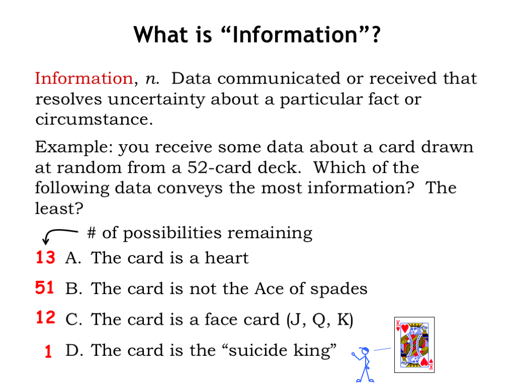
Let’s start by asking “what is information?” From our engineering perspective, we’ll define information as data communicated or received that resolves uncertainty about a particular fact or circumstance. In other words, after receiving the data we’ll know more about that particular fact or circumstance. The greater the uncertainty resolved by the data, the more information the data has conveyed.

Let’s look at an example: a card has been chosen at random from a normal deck of 52 playing cards. Without any data about the chosen card, there are 52 possibilities for the type of the card. Now suppose you receive one of the following pieces of data about the choice.

You learn the suit of the card is Heart. This narrows the choice to down to one of 13 cards.
You learn instead the card is not the Ace of Spades. This still leaves 51 cards that it might be.
You learn instead that the card is a face card, that is, a Jack, Queen or King. So the choice is one of 12 cards.
You learn instead that the card is the suicide king. This is actually a particular card: the King of Hearts where the king is sticking the sword through his head. No uncertainty here! We know exactly what the choice was.

Which of the possible pieces of data conveys the most information? In other words, which data resolves the most uncertainty about the chosen card? Similarly, which data conveys the least amount of information? We’ll answer these questions in the next section.

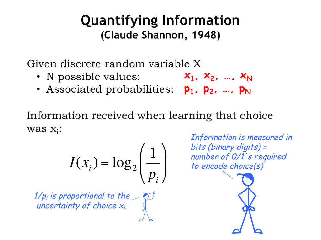
Mathematicians like to model uncertainty about a particular circumstance by introducing the concept of a random variable. For our application, we’ll always be dealing with circumstances where there are a finite number N of distinct choices, so we’ll be using a discrete random variable \(X\) that can take on one of the N possible values from the set \(\{x_1, x_2, ..., x_N\}\). The probability that \(X\) will take on the value \(x_1\) is given by the probability \(p_1\), the value \(x_2\) by probability \(p_2\), and so on. The smaller the probability, the more uncertain it is that \(X\) will take on that particular value.

Claude Shannon, in his seminal work on the theory of information, defined the information received when learning that \(X\) had taken on the value \(x_i\) as \[\begin{equation} I(x_i)=\log_2 \frac{1}{p_i} \textrm{bits}. \end{equation}\] Note that the uncertainty of a choice is inversely proportional its probability, so the term inside of the log is basically the uncertainty of that particular choice. We use the \(\log_2\) to measure the magnitude of the uncertainty in bits where a bit is a quantity that can take on the value 0 or 1. Think of the information content as the number of bits we would require to encode this choice.

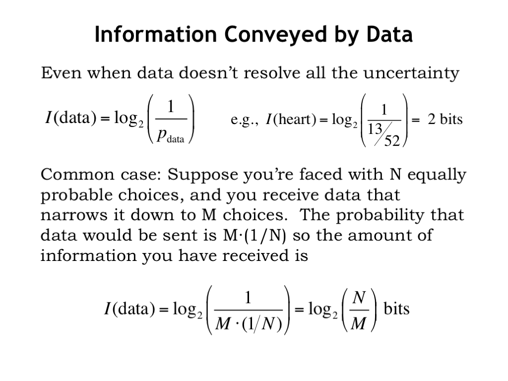
Suppose the data we receive doesn’t resolve all the uncertainty. For example, when earlier we received the data that the card was a Heart: some of uncertainty has been resolved since we know more about the card than we did before the receiving the data, but we don’t yet know the exact card, so some uncertainty still remains. We can slightly modify Equation (1) as follows \[\begin{equation} I(\textrm{data})=\log_2\frac{1}{p_{\textrm{data}}} \textrm{ bits}. \end{equation}\] In our example, the probability of learning that a card chosen randomly from a 52-card deck is a Heart is \(13/52 = 0.25\), the number of Hearts over the total number of choices. So the information content is computed as \[\begin{equation*} I(\textrm{heart}) = \log_2\frac{1}{p_{\textrm{heart}}} = \log_2 \frac{1}{0.25} = 2 \textrm{ bits}. \end{equation*}\]

This example is one we encounter often: we receive partial information about \(N\) equally-probable choices (each choice has probability \(1/N\)) that narrows the number of choices down to \(M\). The probability of receiving such information is \(M(1/N)\), so the information content is \[\begin{equation} I(\textrm{N choices \(\rightarrow\) M choices}) = \log_2 \frac{1}{M(1/N)} = \log_2 \frac{N}{M} \textrm{ bits}. \end{equation}\]

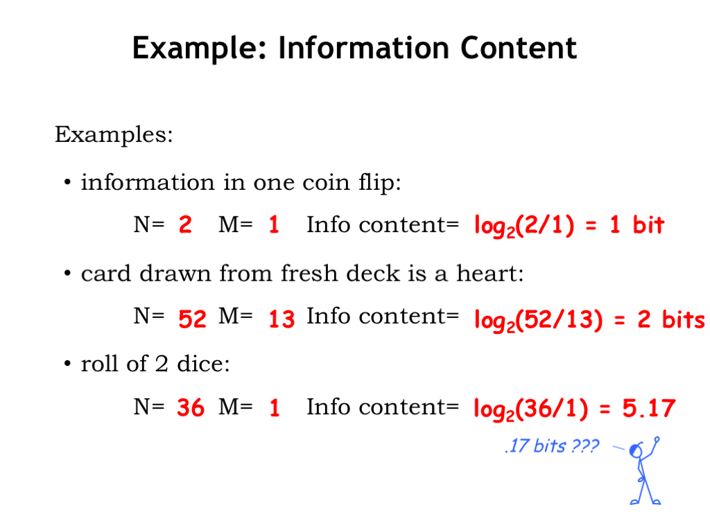
Let’s look at some examples.

If we learn the result (heads or tails) of a flip of a fair coin, we go from 2 choices to a single choice. So, using our equation, the information received is \(\log_2(2/1) = 1\) bit. This makes sense: it would take us one bit to encode which of the two possibilities actually happened, say, “1” for heads and “0” for tails.
Reviewing the example from earlier, learning that a card drawn from a fresh deck is a Heart gives us \(\log_2(52/13) = 2\) bits of information. Again this makes sense: it would take us two bits to encode which of the four possible card suits had turned up.
Finally consider what information we get from rolling two dice, one red and one green. Each die has six faces, so there are 36 possible combinations. Once we learn the exact outcome of the roll, we’ve received \(\log_2(36/1) = 5.17\) bits of information.

Hmm. What do those fractional bits mean? Our digital system only deals in whole bits! So to encode a single outcome, we’d need to use 6 bits. But suppose we wanted to record the outcome of 10 successive rolls. At 6 bits/roll we would need a total of 60 bits. What this formula is telling us is that we would need not 60 bits, but only 52 bits to unambiguously encode the results. Whether we can come up with an encoding that achieves this lower bound is an interesting question that we’ll take up later in this chapter.

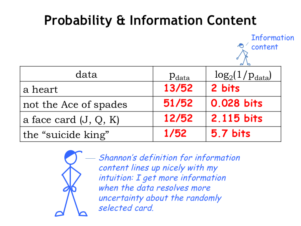
To wrap up, let’s return to our initial example. Here’s a table showing the different choices for the data received, along with the probability of that event and the computed information content.

The results line up nicely with our intuition: the more uncertainty is resolved by the data, the more information we have received. We can use Equation (2) to provide an exact answer to the questions at the end of the first slide. We get the most information when we learn that the card is the suicide King and the least information when we learn that the card is not the Ace of Spades.

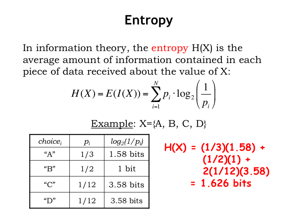
In the next section we’re going to start our discussion on how to actually engineer the bit encodings we’ll use to encode information, but first we’ll need a way to evaluate the efficacy of an encoding. The entropy, \(H(X)\), of a discrete random variable \(X\) is average amount of information received when learning the value of \(X\):

\[\begin{equation} \label{eq:entropy} H(X) = E(I(X)) = \sum_i p_i \log_2 \frac{1}{p_i} \end{equation}\] Shannon followed Boltzmann’s lead in using \(H\), the upper-case variant of the Greek letter \(\eta\) (eta), for “entropy” since \(E\) was already used for “expected value,” the mathematicians’ name for “average.” We compute the expected value in the usual way: we take the weighted sum, where the amount of information received when learning of a particular choice \(i\), \(log_2(1/p_i)\) is weighted by the probability of that choice actually happening.

Here’s an example. We have a random variable that can take on one of four values \(\{A,B,C,D\}\). The probabilities of each choice are shown in the table, along with the associated information content.

Now we’ll compute the entropy using Equation (4): \[\begin{equation*} \begin{split} H(X) & = (1/3)(1.58) + (1/2)(1) + (1/12)(3.58) + (1/12)(3.58) \\ & = 1.626 \textrm{ bits.} \end{split} \end{equation*}\] This is telling us that a clever encoding scheme should, on the average, be able to do better than simply encoding each symbol using 2 bits to represent which of the four possible values is next. Food for thought! We’ll discuss this further in our discussion of variable-length encodings.

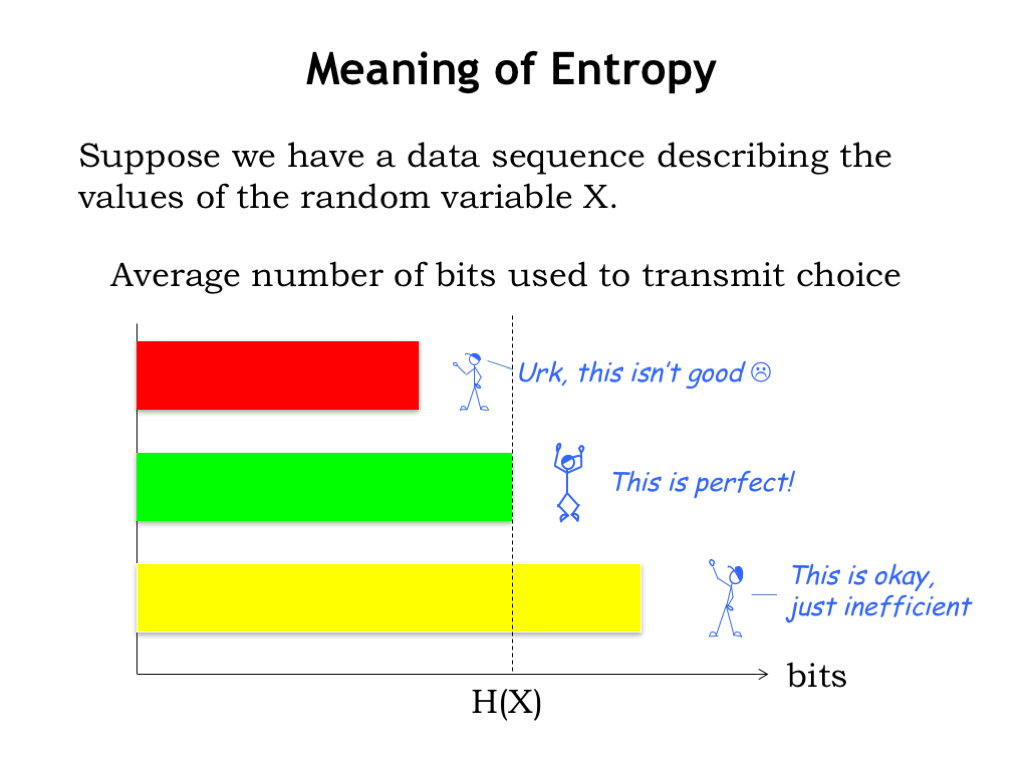
So, what is the entropy telling us? Suppose we have a sequence of data describing a sequence of values of the random variable \(X\).

If, on the average, we use less than \(H(X)\) bits transmit each piece of data in the sequence, we will not be sending enough information to resolve the uncertainty about the values. In other words, the entropy is a lower bound on the number of bits we need to transmit. Getting less than this number of bits wouldn’t be good if the goal was to unambiguously describe the sequence of values — we’d have failed at our job!

On the other hand, if we send, on the average, more than \(H(X)\) bits to describe the sequence of values, we will not be making the most effective use of our resources, since the same information might have been able to be represented with fewer bits. This okay, but perhaps with some insights we could do better.

Finally, if we send on the average exactly \(H(X)\) bits then we’d have the perfect encoding. Alas, perfection is, as always, a tough goal, so most of the time we’ll have to settle for getting close.

Next we turn our attention to encoding data as sequences of 0’s and 1’s, i.e., a string of bits. An encoding is an unambiguous mapping between bit strings and the members of the set of data to be encoded.

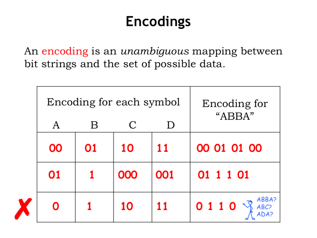
For example, suppose we have a set of four symbols \(\{A,B,C,D\}\) and we want to use bit strings to encode messages constructed of these symbols, e.g., “ABBA.” If we choose to encode the message one character at a time, our encoding would assign a unique bit string to each symbol. The figure above shows some trial encodings.

Since we have four symbols, we might choose a unique two-bit string for each: “A” could be “00,” B = “01,” C = “10,” and D = “11,” as shown in the first encoding in the figure above. This is called a fixed-length encoding since the bit strings used to represent the symbols all have the same length. The encoding for the message “ABBA” would be “00 01 01 00”. And we can run the process backwards: given a bit string and the encoding key, we can look up the next bits in the bit string, using the key to determine the symbol they represent. “00” would be decoded as “A,” “01” as B and so on.

As shown in the second encoding in the table, we can use a variable-length encoding, where the symbols are encoded using bit strings of different lengths. here “A” is encoded as “01,” “B” as “1”, “C” as “000” and “D” = “001.”. “ABBA” would be encoded as “01 1 1 01.” We’ll see that carefully constructed variable-length encodings are useful for the efficient encoding of messages where the symbols occur with different probabilities.

Finally consider the third encoding in the table. We have to be careful that the encoding is unambiguous! Using this encoding, “ABBA” would be encoded as “0 1 1 0.” Looking good since that encoding is shorter than either of the previous two encodings. Now let’s try to decode this bit string — oops. Using the encoding key, we can unfortunately arrive at several decodings: “ABBA” of course, but also “ADA” or “ABC” depending on how we group the bits. This attempt at specifying an encoding has failed since the message cannot be interpreted unambiguously.

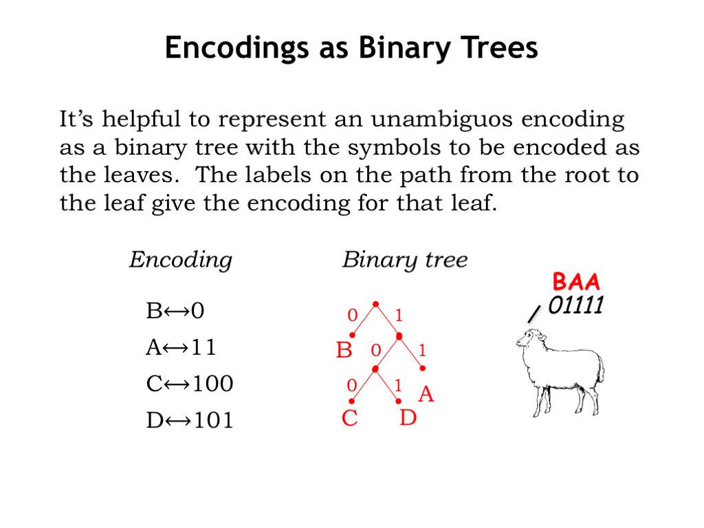
Graphically we can represent an unambiguous encoding as a binary tree, labeling the branches from each tree node with “0” and “1,” placing the symbols to be encoded as the leaves of the tree. If you build a binary tree for a proposed encoding and find that there are no symbols labeling interior nodes and exactly one symbol at each leaf, then your encoding is good to go!

For example, consider the encoding shown on the left of the figure. It just takes a second to draw the corresponding binary tree. The symbol “B” is distance 1 from the root of the tree, along an arc labeled “0”. “A” is distance two, and “C” and “D” are distance 3.

If we receive an encoded message, e.g., “01111,” we can decode it by using successive bits of the encoding to identify a path from the root of tree, descending step-by-step until we come to leaf, then repeating the process starting at the root again, until all the bits in the encoded message have been consumed. So the message from the sheep is decoded as follows:

“0” takes us from the root to the leaf “B”, which is our first decoded symbol.
Then “1-1” takes us to “Ak” and
the next “1-1” results in a second “A.”

The final decoded message, “BAA,” is not totally unexpected, at least from an American sheep.

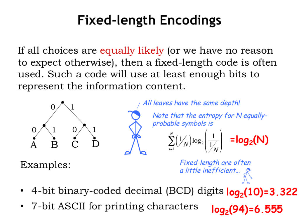
If the symbols we are trying to encode occur with equal probability (or if we have no a priori reason to believe otherwise), then we’ll use a fixed-length encoding, where all leaves in the encoding’s binary tree are the same distance from the root. Fixed-length encodings have the advantage of supporting random access, where we can figure out the Nth symbol of the message by simply skipping over the required number of bits. For example, in a message encoded using the fixed-length code shown here, if we wanted to determine the third symbol in the encoded message, we would skip the 4 bits used to encode the first two symbols and start decoding with the 5th bit of message.

Mr. Blue is telling us about the entropy for random variables that have N equally-probable outcomes. In this case, each element of the sum in the entropy formula is simply \((1/N)*\log_2(N)\), and, since there are N elements in the sequence, the resulting entropy is just \(\log_2(N)\).

Let’s look at some simple examples. In binary-coded decimal, each digit of a decimal number is encoded separately. Since there are 10 different decimal digits, we’ll need to use a 4-bit code to represent the 10 possible choices. The associated entropy is \(\log_2(10)\), which is 3.322 bits. We can see that our chosen encoding is inefficient in the sense that we’d use more than the minimum number of bits necessary to encode, say, a number with 1000 decimal digits: our encoding would use 4000 bits, although the entropy suggests we *might* be able to find a shorter encoding, say, 3400 bits, for messages of length 1000.

Another common encoding is ASCII, the code used to represent English text in computing and communication. ASCII has 94 printing characters, so the associated entropy is \(\log_2(94)\) or 6.555 bits, so we would use 7 bits in our fixed-length encoding for each character.

One of the most important encodings is the one we use to represent numbers. Let’s start by thinking about a representation for unsigned integers, numbers starting at 0 and counting up from there. Drawing on our experience with representing decimal numbers, i.e., representing numbers in base 10 using the 10 decimal digits, our binary representation of numbers will use a base 2 representation using the two binary digits.

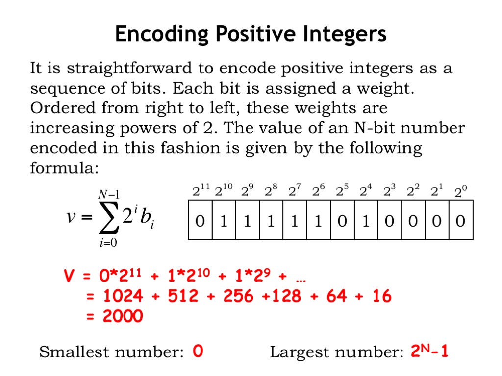
The formula for converting an N-bit binary representation of a numeric value into the corresponding integer is shown below — just multiply each binary digit by its corresponding weight in the base-2 representation. For example, here’s a 12-bit binary number, with the weight of each binary digit shown above. We can compute its value as \(0*2^{11}\) plus \(1*2^{10}\) plus \(1*2^9\), and so on. Keeping only the non-zero terms and expanding the powers-of-two gives us the sum

1024 + 512 + 256 + 128 + 64 + 16

which, expressed in base-10, sums to the number 2000.

With this N-bit representation, the smallest number that can be represented is 0 (when all the binary digits are 0) and the largest number is \(2^N - 1\) (when all the binary digits are 1). Many digital systems are designed to support operations on binary-encoded numbers of some fixed size, e.g., choosing a 32-bit or a 64-bit representation, which means that they would need multiple operations when dealing with numbers too large to be represented as a single 32-bit or 64-bit binary string.

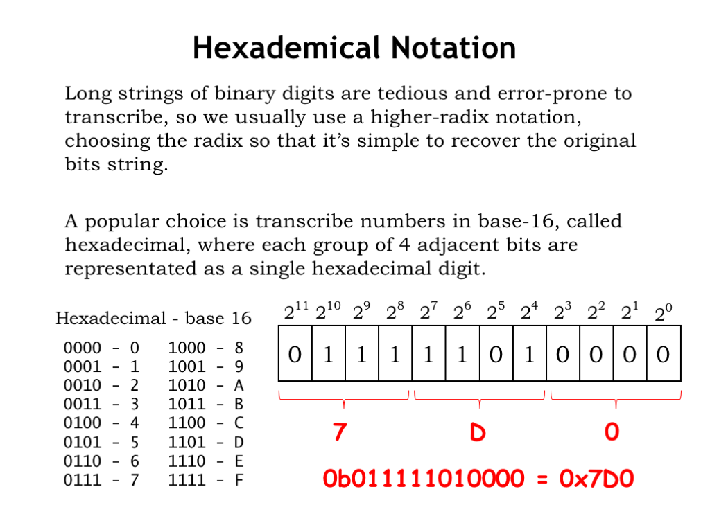
Long strings of binary digits are tedious and error-prone to transcribe, so let’s find a more convenient notation, ideally one where it will be easy to recover the original bit string without too many calculations. A good choice is to use a representation based on a radix that’s some higher power of 2, so each digit in our representation corresponds to some short contiguous string of binary bits. A popular choice these days is a radix-16 representation, called hexadecimal or “hex” for short, where each group of 4 binary digits is represented using a single hex digit.

Since there are 16 possible combinations of 4 binary bits, we’ll need 16 hexadecimal digits: we’ll borrow the ten digits “0” through “9” from the decimal representation, and then simply use the first six letters of the alphabet, “A” through “F” for the remaining digits. The translation between 4-bit binary and hexadecimal is shown in the table to the left below.

To convert a binary number to hex, group the binary digits into sets of 4, starting with the least-significant bit (that’s the bit with weight \(2^0\)). Then use the table to convert each 4-bit pattern into the corresponding hex digit: “0000” is the hex digit “0”, “1101” is the hex digit “D,” and “0111” is the hex digit “7”. The resulting hex representation is “7D0.” To prevent any confusion, we’ll use a special prefix “0x” to indicate when a number is being shown in hex, so we’d write “0x7D0” as the hex representation for the binary number “0111 1101 0000.” This notation convention is used by many programming languages for entering binary bit strings.

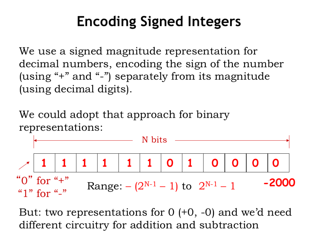
Our final challenge is figuring out how to represent signed integers, e.g., what should be our representation for the number -2000?

In decimal notation, the convention is to precede the number with a “+” or “-” to indicate whether it’s positive or negative, usually omitting the “+” to simplify the notation for positive numbers. We could adopt a similar notation — called signed magnitude — in binary, by allocating a separate bit at the front of the binary string to indicate the sign, say “0” for positive numbers and “1” for negative numbers. So the signed-magnitude representation for -2000 would be an initial “1” to indicate a negative number, followed by the representation for 2000 (as described on the previous two slides).

However there are some complications in using a signed-magnitude representation. There are two possible binary representations for zero: “+0” and “-0”. This makes the encoding slightly inefficient but, more importantly, the circuitry for doing addition of signed-magnitude numbers is different than the circuitry for doing subtraction. Of course, we’re used to that — in elementary school we learned one technique for addition and another for subtraction.

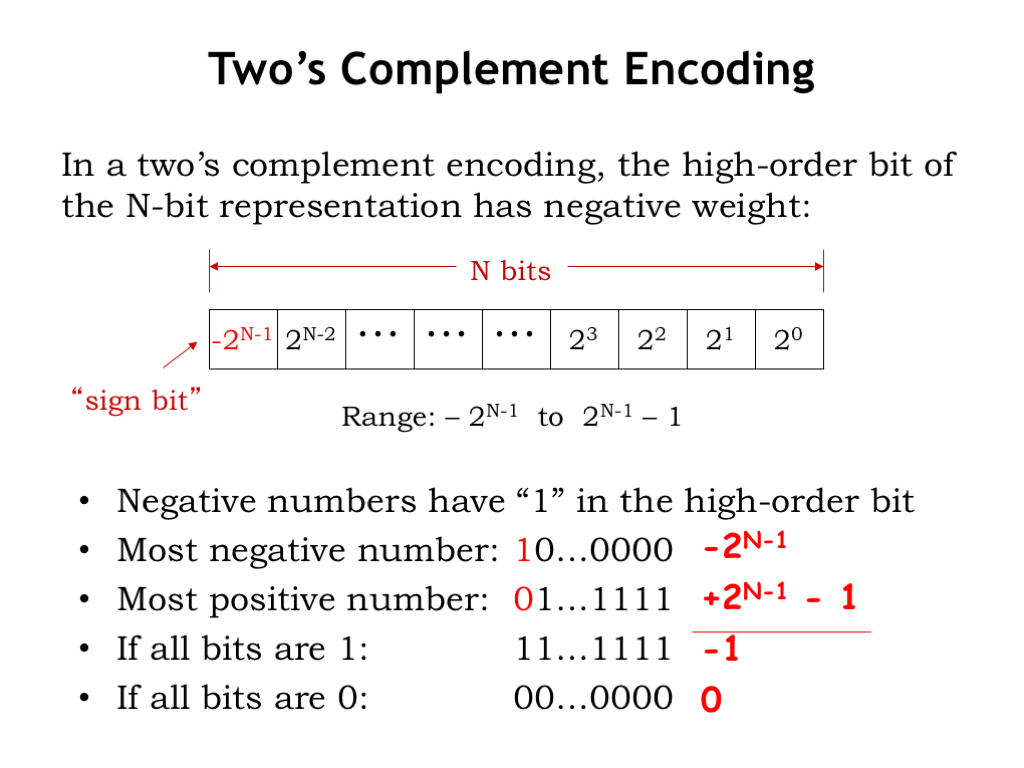
To keep the circuitry simple, most modern digital systems use the two’s complement binary representation for signed integers. In this representation, the high-order bit of an N-bit two’s complement number has a negative weight, as shown in the figure. Thus all negative numbers have a 1 in the high-order bit and, in that sense, the high-order bit is serving as the sign bit — if it’s 1, the represented number is negative.

The most negative N-bit number has a 1-bit in the high-order position, representing the value \(-2^{N-1}\). The most positive N-bit number has a 0 in the negative-weight high-order bit and 1’s for all the positive-weight bits, representing the value \(2^{N-1}-1\). This gives us the range of possible values, e.g., in an 8-bit two’s complement representation, the most negative number is \(-2^7 = -128\) and the most positive number is \(2^7 - 1 = 127\).

If all N bits are 1, think of that as the sum of the most negative number with the most positive number, i.e., \(-2^{N-1} + 2^{N-1}-1\), which equals -1. And, of course, if all N bits are 0, that’s the unique representation of 0.

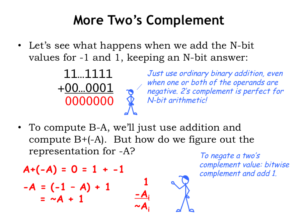
Let’s see what happens when we add the N-bit values for -1 and 1, keeping an N-bit answer. In the rightmost column, 1 plus 1 is 0, carry the 1. In the second column, the carry of 1 plus 1 plus 0 is 0, carry the 1. And so on — the result is all zero’s, the representation for 0... perfect! Notice that we just used ordinary binary addition, even when one or both of the operands are negative. Two’s complement is perfect for N-bit arithmetic!

To compute B - A, we can just use addition and compute B + (-A). So now we just need to figure out the two’s complement representation for -A, given the two’s complement representation for A. Well, we know that A + (-A) = 0 and using the example above, we can rewrite 0 as 1 + (-1). Reorganizing terms, we see that -A equals 1 plus the quantity (-1) - A. As we saw above, the two’s complement representation for -1 is all 1-bits, so we can write that subtraction as all 1’s minus the individual bits of A: \(A_0\), \(A_1\), ... up to \(A_{N-1}\). If a particular bit \(A_i\) is 0, then \(1-A_i = 1\) and if \(A_i\) is 1, then \(1-A_i = 0\). So in each column, the result is the bitwise complement of \(A_i\), which we’ll write using the C-language bitwise complement operator tilde. So we see that -A equals the bitwise complement of A plus 1. Ta-dah!

To practice your skill with two’s complement, try your hand at the following exercises. All you need to remember is how to do binary addition and two’s complement negation (which is bitwise complement and add 1).

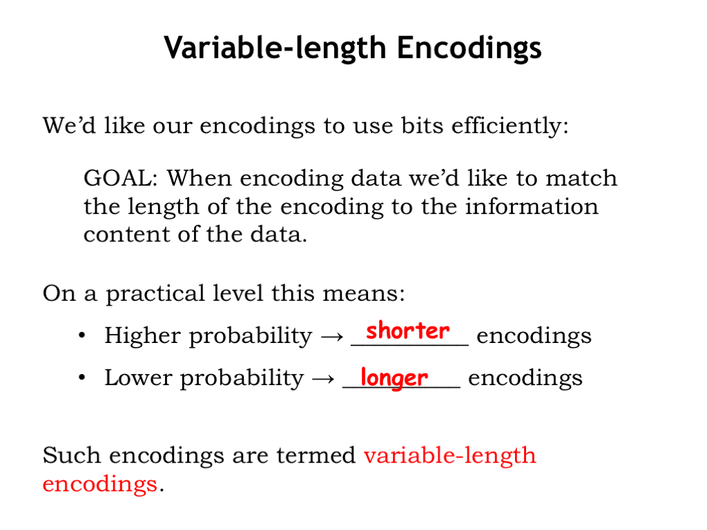
Fixed-length encodings work well when all the possible choices have the same information content, i.e., all the choices have an equal probability of occurring. If those choices don’t have the same information content, we can do better. To see how, consider the expected length of an encoding, computed by considering each \(x_i\) to be encoded, and weighting the length of its encoding by \(p_i\), the probability of its occurrence. By “doing better” we mean that we can find encodings that have a shorter expected length than a fixed-length encoding. Ideally we’d like the expected length of the encoding for the \(x_i\) to match the entropy H(X), which is the expected information content.

We know that if \(x_i\) has a higher probability (i.e., a larger \(p_i\)), that is has a smaller information content, so we’d like to use shorter encodings. If \(x_i\) has a lower probability, then we’d use a longer encoding.

So we’ll be constructing encodings where the \(x_i\) may have different length codes — we call these variable-length encodings.

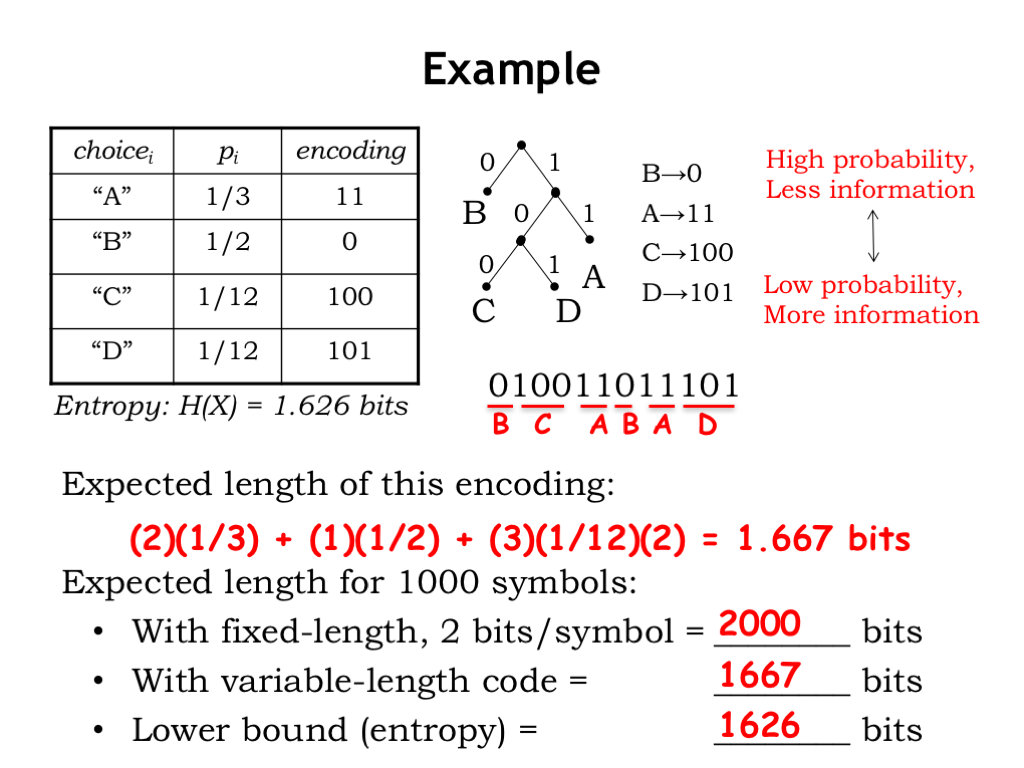
Here’s an example we’ve seen before. There are four possible choices to encode (A, B, C, and D), each with the specified probability. The table shows a suggested encoding where we’ve followed the advice from the previous slide: high-probability choices that convey little information (e.g., B) are given shorter encodings, while low-probability choices that convey more information (e.g., C or D) are given longer encodings.

Let’s diagram this encoding as a binary tree. Since the symbols all appear as the leaves of the tree, we can see that the encoding is unambiguous. Let’s try decoding the following encoded data. We’ll use the tree as follows: start at the root of the tree and use bits from the encoded data to traverse the tree as directed, stopping when we reach a leaf.

Starting at the root, the first encoded bit is 0, which takes us down the left branch to the leaf B. So B is the first symbol of the decoded data. Starting at the root again, 1 takes us down the right branch, 0 the left branch from there, and 0 the left branch below that, arriving at the leaf C, the second symbol of the decoded data. Continuing on: 11 gives us A, 0 decodes as B, 11 gives us A again, and, finally, 101 gives us D. The entire decoded message is “BCABAD.”

The expected length of this encoding is easy to compute: the length of A’s encoding (2 bits) times its probability (1/3), plus the length of B’s encoding (1 bit) times 1/2, plus the contributions for C and D, each 3 times 1/12. This adds up to 1 and 2/3 bits.

How did we do? If we had used a fixed-length encoding for our four possible symbols, we’d have needed 2 bits each, so we’d need 2000 bits to encode 1000 symbols. Using our variable-length encoding, the expected length for 1000 symbols would be 1667. The lower bound on the number of bits needed to encode 1000 symbols is 1000 times the entropy H(X), which is 1626 bits, so the variable-length code got us closer to our goal, but not quite all the way there.

Could another variable-length encoding have done better? In general, it would be nice to have a systematic way to generate the best-possible variable-length code, and that’s the subject of the next video.

Given a set of symbols and their probabilities, Huffman’s Algorithm tells us how to construct an optimal variable-length encoding. By “optimal” we mean that, assuming we’re encoding each symbol one-at-a-time, no other variable-length code will have a shorter expected length.

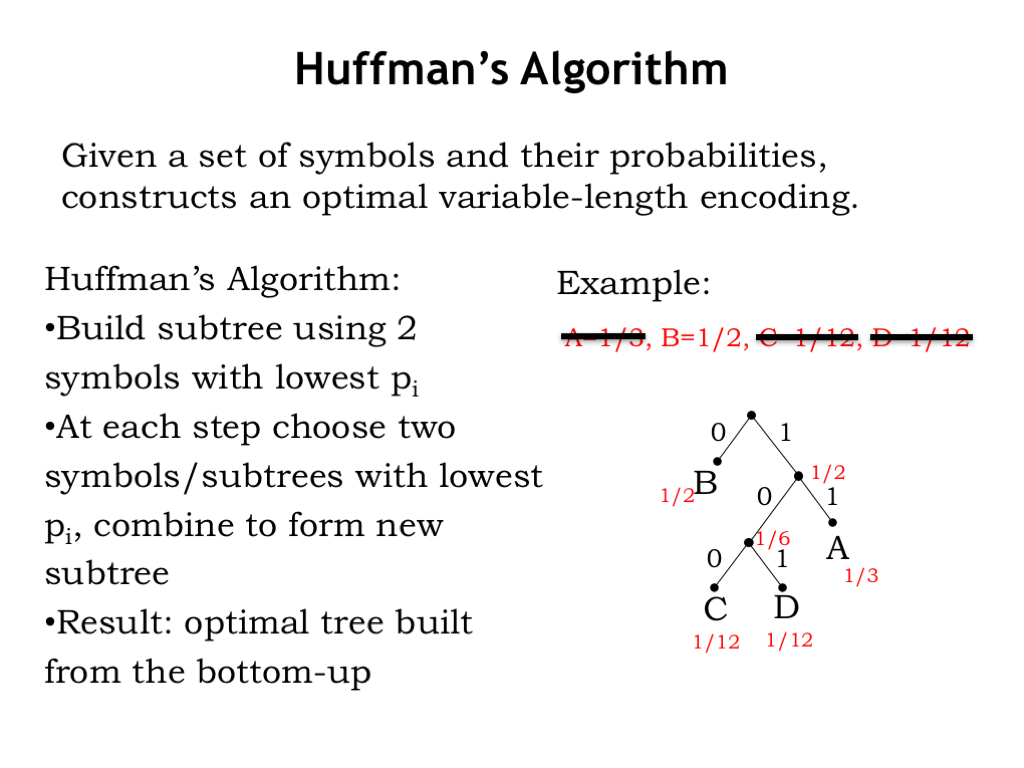
The algorithm builds the binary tree for the encoding from the bottom up. Start by choosing the two symbols with the smallest probability (which means they have highest information content and should have the longest encoding). If anywhere along the way, two symbols have the same probability, simply choose one arbitrarily. In our running example, the two symbols with the lowest probability are C and D.

Combine the symbols as a binary subtree, with one branch labeled “0” and the other “1.” It doesn’t matter which labels go with which branch. Remove C and D from our list of symbols, and replace them with the newly constructed subtree, whose root has the associated probability of 1/6, the sum of the probabilities of its two branches.

Now continue, at each step choosing the two symbols and/or subtrees with the lowest probabilities, combining the choices into a new subtree. At this point in our example, the symbol A has the probability 1/3, the symbol B the probability 1/2 and the C/D subtree probability 1/6. So we’ll combine A with the C/D subtree.

On the final step we only have two choices left: B and the A/C/D subtree, which we combine in a new subtree, whose root then becomes the root of the tree representing the optimal variable-length code. Happily, this is the code we’ve been using all along!

As mentioned above, we can produce a number of different variable-length codes by swapping the “0” and “1” labels on any of the subtree branches. But all those encodings would have the same expected length, which is determined by the distance of each symbol from the root of the tree, not the labels along the path from root to leaf. So all these different encodings are equivalent in terms of their efficiency.

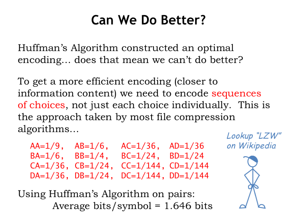
“Optimal” sounds pretty good! Does that mean we can’t do any better? Well, not by encoding symbols one-at-a-time. But if we want to encode long sequences of symbols, we can reduce the expected length of the encoding by working with, say, pairs of symbols instead of only single symbols. The table below shows the probability of pairs of symbols from our example. If we use Huffman’s Algorithm to build the optimal variable-length code using these probabilities, it turns out the expected length when encoding pairs is 1.646 bits/symbol. This is a small improvement on the 1.667 bits/symbols when encoding each symbol individually. And we’d do even better if we encoded sequences of length 3, and so on.

Modern file compression algorithms use an adaptive algorithm to determine on-the-fly which sequences occur frequently and hence should have short encodings. They work quite well when the data has many repeating sequences, e.g., natural language data where some letter combinations or even whole words occur again and again. Compression can achieve dramatic reductions from the original file size. If you’d like to learn more, look up “LZW” on Wikipedia to read the Lempel-Ziv-Welch data compression algorithm.

Now let’s think a bit about what happens if there’s an error and one or more of the bits in our encoded data gets corrupted. We’ll focus on single-bit errors, but much of what we discuss can be generalized to multi-bit errors.

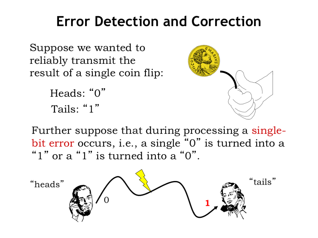
For example, consider encoding the results from some unpredictable event, e.g., flipping a fair coin. There are two outcomes: heads, encoded as, say, 0, and tails encoded as 1. Now suppose some error occurs during processing, e.g., the data is corrupted while being transmitted from Bob to Alice: Bob intended to send the message heads, but the 0 was corrupted and become a 1 during transmission, so Alice receives 1, which she interprets as tails. Note that Alice can’t distinguish between receiving a message of heads that has an error and an uncorrupted message of tails — she cannot detect that an error has occurred. So this simple encoding doesn’t work very well if there’s the possibility of single-bit errors.

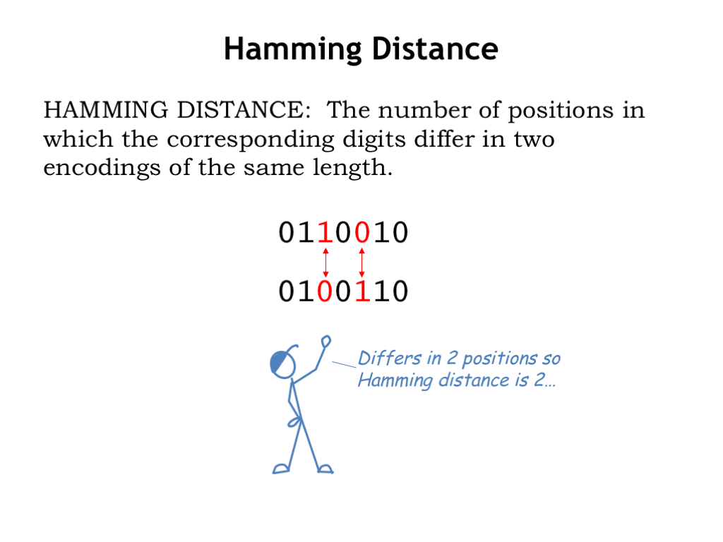
To help with our discussion, we’ll introduce the notion of Hamming distance, defined as the number of positions in which the corresponding digits differ in two encodings of the same length. For example, here are two 7-bit encodings, which differ in their third and fifth positions, so the Hamming distance between the encodings is 2. If someone tells us the Hamming distance of two encodings is 0, then the two encodings are identical. Hamming distance is a handy tool for measuring how to encodings differ.

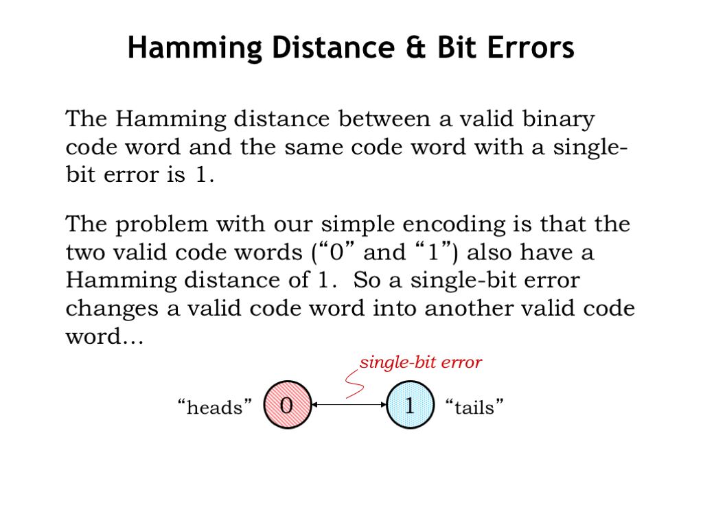
How does this help us think about single-bit errors? A single-bit error changes exactly one of the bits of an encoding, so the Hamming distance between a valid binary code word and the same code word with a single-bit error is 1.

The difficulty with our simple encoding is that the two valid code words (“0” and “1”) also have a Hamming distance of 1. So a single-bit error changes one valid code word into another valid code word. We’ll show this graphically, using an arrow to indicate that two encodings differ by a single bit, i.e., that the Hamming distance between the encodings is 1.

The real issue here is that when Alice receives a 1, she can’t distinguish between an uncorrupted encoding of tails and a corrupted encoding of heads — she can’t detect that an error occurred. Let’s figure how to solve her problem!

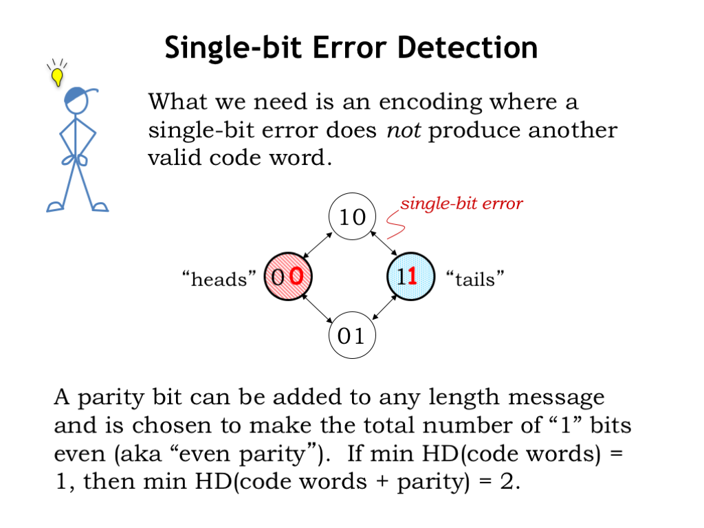
The insight is to come up with a set of valid code words such that a single-bit error does NOT produce another valid code word. What we need are code words that differ by at least two bits, i.e., we want the minimum Hamming distance between any two code words to be at least 2.

If we have a set of code words where the minimum Hamming distance is 1, we can generate the set we want by adding a parity bit to each of the original code words. There’s even parity and odd parity — using even parity, the additional parity bit is chosen so that the total number of 1 bits in the new code word are even.

For example, our original encoding for heads was 0, adding an even parity bit gives us 00. Adding an even parity bit to our original encoding for tails gives us 11. The minimum Hamming distance between code words has increased from 1 to 2.

How does this help? Consider what happens when there’s a single-bit error: 00 would be corrupted to 01 or 10, neither of which is a valid code word — aha! we can detect that a single-bit error has occurred. Similarly single-bit errors for 11 would also be detected. Note that the valid code words 00 and 11 both have an even number of 1-bits, but that the corrupted code words 01 or 10 have an odd number of 1-bits. We say that corrupted code words have a parity error.

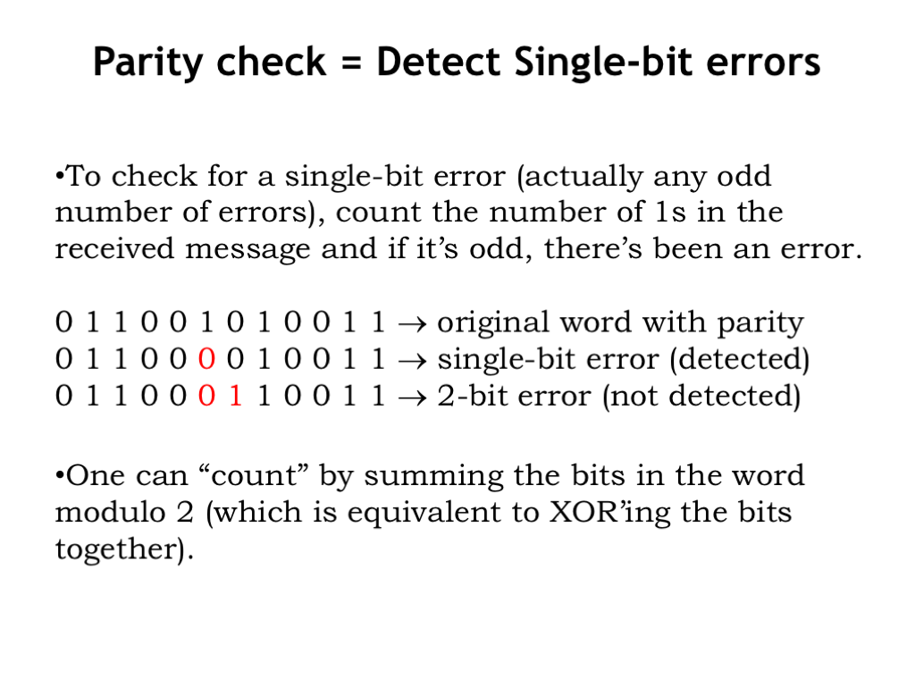
It’s easy to perform a parity check: simply count the number of 1s in the code word. If it’s even, a single-bit error has NOT occurred; if it’s odd, a single-bit error HAS occurred. We’ll see in a couple of chapters that the Boolean function exclusive-or can be used to perform parity checks.

Note that parity won’t help us if there’s an even number of bit errors, where a corrupted code word would have an even number of 1-bits and hence appear to be okay. Parity is useful for detecting single-bit errors; we’ll need a more sophisticated encoding to detect more errors.

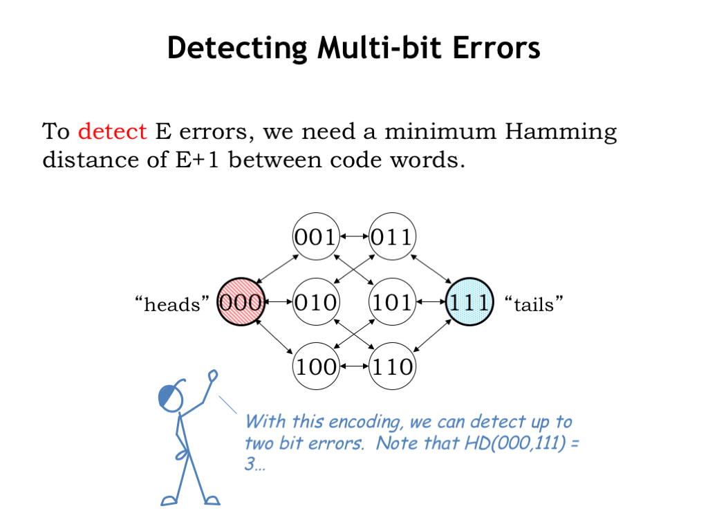
In general, to detect some number \(E\) of errors, we need a minimum Hamming distance of \(E+1\) between code words. We can see this graphically below which shows how errors can corrupt the valid code words 000 and 111, which have a Hamming distance of 3. In theory this means we should be able to detect up to 2-bit errors.

Each arrow represents a single-bit error and we can see from the diagram that following any path of length 2 from either 000 or 111 doesn’t get us to the other valid code word. In other words, assuming we start with either 000 or 111, we can detect the occurrence of up to 2 errors.

Basically our error detection scheme relies on choosing code words far enough apart, as measured by Hamming distance, so that \(E\) errors can’t corrupt one valid code word so that it looks like another valid code word.

Is there any chance we can not only detect a single-bit error but also correct the error to recover the original data? Sure! Here’s how.

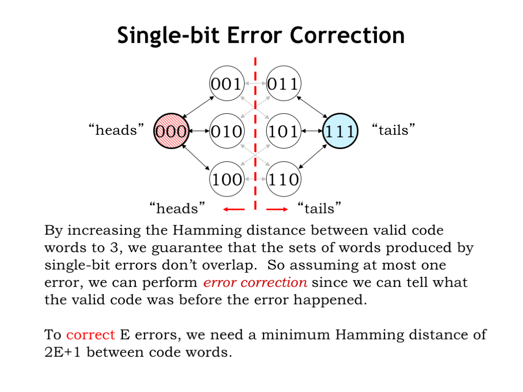
By increasing the Hamming distance between valid code words to 3, we guarantee that the sets of code words produced by single-bit errors don’t overlap. The set of code words produced by corrupting 000 (100, 010, or 001) has no code words in common with the set of code words produced by corrupting 111 (110, 101, or 011). Assuming that at most one error occurred, we can deduce the original code word from whatever code word we receive. For example if we receive 001, we deduce that the original code word was 000 and there has been a single-bit error.

Again we can generalize this insight: if we want to correct up to \(E\) errors, the minimum Hamming distance between valid code words must be at least \(2E + 1\). For example, to correct single-bit errors we need valid code words with a minimum Hamming distance of 3.

Coding theory is a research area devoted to developing algorithms to generate code words that have the necessary error detection and correction properties. You can take entire courses on this topic! But we’ll stop here with our basic insights: by choosing code words far enough apart (as measured by Hamming distance) we can ensure that we can detect and even correct errors that have corrupted our encoded data. Pretty neat!

1.1 Annotated Slides

L01: Basics of Information